
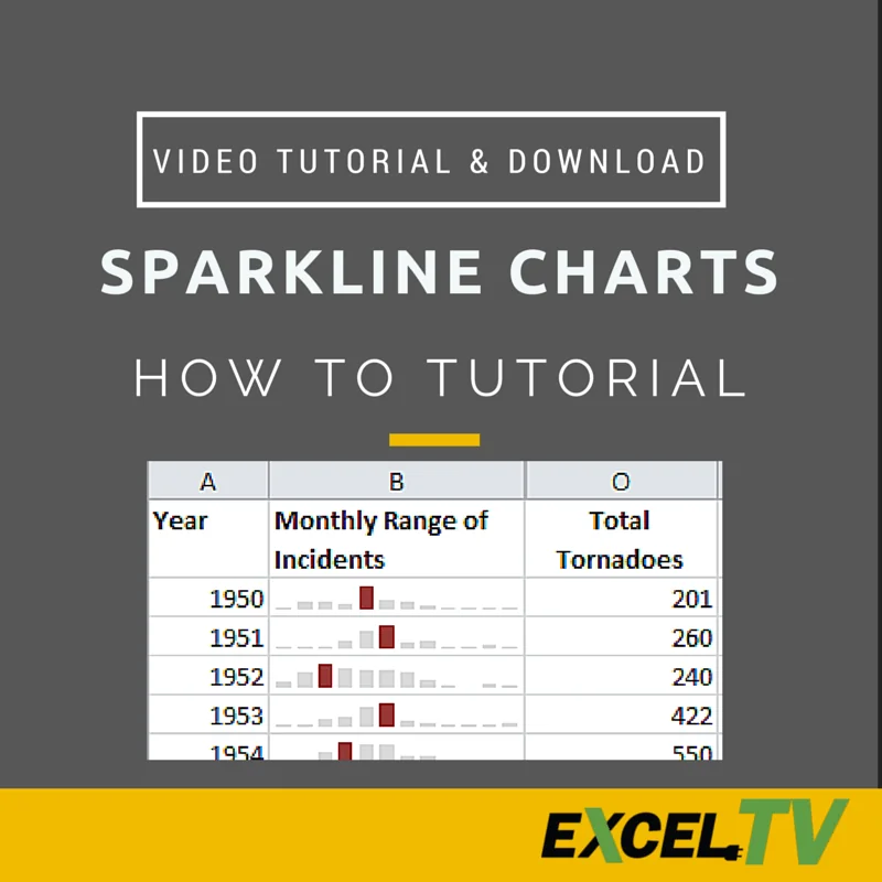
To add a sparkline in Excel, select the cell where the tiny chart should appear, go to Insert > Sparklines, choose Line, Column, or Win/Loss, then select the source data range. Sparklines are miniature charts inside worksheet cells, useful when you want a compact trend next to each row of data.
Use sparklines when a full chart would take too much space. They work especially well in dashboards, scorecards, monthly reports, and tables where each row needs a quick visual cue. For larger chart layouts, use a full Excel chart instead, such as a data visualization chart or a more advanced 3D chart setup.
Step 1: Prepare the Data
Put your source values in a clean row or column. A sparkline needs a simple series, such as monthly sales, weekly tickets, inventory levels, or profit/loss outcomes.
For a row-based report, keep the data values across the row and place the sparkline in the next blank cell. For a column-based report, put the sparkline below or beside the source range.
Good source data for sparklines:
- Monthly revenue by product
- Weekly support-ticket counts
- Daily website visits
- Profit/loss results by period
- Budget variance by department
If your data is messy, clean it first. For example, use Power Query in Excel before creating a dashboard table that depends on consistent source values.
Step 2: Insert a Line Sparkline
Use a Line sparkline when the shape of the trend matters more than the size of each individual value. Line sparklines are the best default for time-series data because the viewer can quickly see direction, peaks, dips, and volatility.
To insert one:
- Select the blank cell where the sparkline should appear.
- Go to Insert > Sparklines > Line.
- Select the source data range.
- Confirm the location range and click OK.
Use Line sparklines for sales over time, customer counts, traffic trends, or any row where the order of the values matters.
Step 3: Insert a Column Sparkline
Use a Column sparkline when you want each value to read as a small bar. Column sparklines are better than Line sparklines when the individual value heights matter, such as comparing each month against the rest of the row.
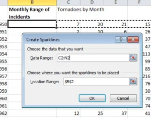
To create one, select the destination cell, go to Insert > Sparklines > Column, select the data range, and press OK.
You will see the sparkline chart appear in the selected cell.
Column sparklines work well for monthly revenue, expense totals, units sold, or any report where the size of each period should be visible without opening a full chart.
Step 4: Insert a Win/Loss Sparkline
Use a Win/Loss sparkline when direction matters more than magnitude. Excel converts each value into a positive, negative, or zero marker, so the chart shows whether each period was a win or a loss.
This type is useful for:
- Profit vs loss by month
- Over-budget vs under-budget results
- Pass/fail quality checks
- Positive vs negative cash-flow periods
To add one, select the destination cell, choose Insert > Sparklines > Win/Loss, select the source range, and click OK. If your values include both positive and negative numbers, the pattern will show immediately.
Step 5: Format Sparkline Colors
Select the sparkline and go to the Sparkline Design tab. Under Style, choose a built-in color scheme, or use Sparkline Color to set the line or bar color directly.
Keep the color simple. A neutral sparkline with one highlighted point is usually easier to read than a row of bright colors. If the sparkline is part of a dashboard, match the color to the surrounding report style.
Step 6: Highlight High, Low, First, Last, and Negative Points
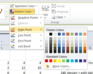
You might want to highlight the highest point in the sparkline. Under Sparkline Design > Show, check High Point. Excel marks the highest value with a separate color.
You can also turn on:
- Low Point for the smallest value
- First Point for the starting value
- Last Point for the ending value
- Negative Points for values below zero
- Markers for each point on Line sparklines
Within Marker Color, choose the color Excel should use for each marker type.
If you already use conditional formatting in Excel, think of sparkline markers the same way: they help the reader find the important parts of the data without studying every number.
Step 7: Set the Axis Scale to Same for All Sparklines
Axis scaling is the easiest sparkline setting to miss. If each sparkline uses its own automatic scale, two rows can look equally strong even when one row has much smaller values. That can mislead the reader.
To use the same scale:
- Select all related sparklines.
- Go to Sparkline Design > Axis.
- Under Vertical Axis Minimum Value Options, choose Same for All Sparklines.
- Under Vertical Axis Maximum Value Options, choose Same for All Sparklines.
Use this setting when the rows are comparable, such as product revenue, monthly costs, or department totals. Keep individual automatic scales only when each row is independent and the trend shape matters more than cross-row comparison.
Step 8: Copy Sparklines Down a Table
Sparkline charts behave much like formulas when you copy and paste them. If your data is in rows and you want one sparkline for each row, create the first sparkline, then copy it down the column.
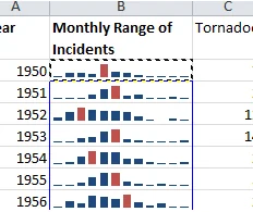
Excel will adjust the source ranges relatively, similar to how copied formulas adjust cell references. Check the first few copied sparklines to confirm that each one points to the correct row.
For larger reports, combine sparklines with tables, filters, and drop-down lists in Excel so users can scan the same metrics from different angles.
Step 9: Show Sparklines When Source Data Is Hidden
Once you have the Sparkline charts of your data, you might want to hide that data.
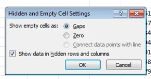
You can group the source columns using the Group tool in the Data tab. After you hide the source data, the sparklines may disappear unless you change one setting.
To keep them visible:
- Select the sparklines.
- Go to Sparkline Design > Edit Data.
- Choose Hidden & Empty Cells.
- Check Show data in hidden rows and columns.
- Click OK.
Now, when your grouped data is minimized or hidden away, the Sparkline charts will still be visible.
When to Use Sparklines Instead of Full Charts
Use sparklines when the chart belongs inside the table. They are ideal for quick scanning, not for detailed presentation.
Choose sparklines when:
- Each row needs its own trend line.
- You have many small series to compare.
- The reader already understands the metric.
- Space is tight.
Choose a full chart when:
- You need axis labels, legends, or annotations.
- The chart will be presented on its own.
- The reader needs exact values.
- The data needs multiple series in one visual.
For presentation-quality visuals, start with a full chart. For dense tables and dashboards, sparklines are usually faster to read.
Get the Download
FAQ
What are the three sparkline types in Excel?
Excel has Line, Column, and Win/Loss sparklines. Line is best for trends, Column is best for magnitude comparisons, and Win/Loss is best for positive/negative outcomes.
Why do my sparklines look misleading?
The most common issue is axis scaling. If each sparkline has its own scale, rows with very different values can look similar. Use Axis > Same for All Sparklines when rows need to be compared.
Can I use sparklines with hidden source data?
Yes. Use Sparkline Design > Edit Data > Hidden & Empty Cells, then enable Show data in hidden rows and columns.
