
Exploring the world of data analysis can be quite fascinating, and using tools like Excel to perform complex simulations makes it even more accessible. A Monte Carlo simulation is one such powerful technique that allows us to model the probability of different outcomes in a process that cannot easily be predicted due to the intervention of random variables.
In Excel, you can perform Monte Carlo simulations to analyze and make informed decisions about uncertain situations. This method involves using random numbers and statistical functions, making Excel a versatile tool for tackling these calculations.
In the video above, Oz asks about the various uses for Monte Carlo Simulation. What have you used it for? Are there any specific examples that you can share with the group? If so, leave a note below in the comments section. Also, feel free to sign up for our newsletter, so that you can stay up to date as new Excel.TV shows are announced. Leave me a message below to stay in contact.
When working with Excel, I find its capabilities for random number generation and probability distribution to be particularly valuable for Monte Carlo simulations. Functions like RAND and NORMINV enable us to create realistic models of possible outcomes by simulating randomness. This makes Excel a practical choice for professionals in fields such as finance, engineering, and project management who need to assess risks and outcomes with greater precision.
For those interested in diving deeper into Monte Carlo simulations, Excel provides a comprehensive platform for both beginners and advanced users. It allows you to visualize your simulation results effectively, offering insights that guide better business decisions. This blend of simplicity and power makes Excel indispensable for anyone looking to leverage the benefits of Monte Carlo simulations.
Key Takeaways
-
Monte Carlo simulations model probabilities using Excel.
-
Excel functions aid in realistic simulation modeling.
-
Results help in informed decision-making.
Fundamentals of Monte Carlo Simulation
Monte Carlo simulation is a powerful tool often used in decision-making processes to evaluate the impact of risk and uncertainty. This method relies on running numerous scenarios to predict possible outcomes across various fields like engineering, project management, and supply chain management.
Conceptual Overview
Monte Carlo simulation is based on probability and random variables. By using random sampling, I can simulate a range of different scenarios. This provides a way to understand the likelihood of various outcomes. The concept hinges on running multiple iterations to cover many possible outcomes, which helps in exploring uncertainties.
The randomness is usually introduced through functions like RAND(), simulating variability. With each iteration, I observe different results influenced by changes in input variables. This offers a comprehensive view of potential risks, making it an effective decision-making tool. Understanding these concepts allows me to make informed predictions about future events and minimize risks.
Applications in Different Industries
In engineering, Monte Carlo methods are used to assess reliability and performance under varying conditions. By modeling different stress scenarios, I can predict equipment failures and optimize maintenance schedules.
In project management, I utilize simulations to plan resources, manage timeframes, and control costs more effectively. By exploring different paths a project might take, I get a clearer picture of potential pitfalls.
In manufacturing and supply chain management, simulations help manage inventory and forecast demand fluctuations. These industries benefit immensely from the insight offered by Monte Carlo methods, allowing me to strategize and ensure smooth operations under uncertainty.
Setting Up a Monte Carlo Simulation in Excel
To successfully set up a Monte Carlo Simulation in Excel, I focus on understanding the problem and building a robust model framework. This involves defining the scope, identifying key variables, and integrating statistical methods to handle uncertainty.
Defining the Problem and Objectives
When I start setting up a Monte Carlo Simulation in Excel, the first step is to clearly define the problem I aim to tackle. I identify the objectives, which could be predicting outcomes or assessing risks. This helps me focus my efforts and set clear goals for my simulation.
I then gather a relevant dataset, ensuring it includes all necessary variables. By understanding the dataset, I can better define the probability distributions that might impact outcomes. It’s important to recognize model uncertainty and plan for it by selecting the right statistical concepts.
Choosing input variables essential to the simulation is another priority. These are the components that I’ll alter during the simulation to observe changes in outcomes. I often make a list of these key variables to ensure a structured approach.
Creating a Model Framework
Creating a solid model framework involves structuring the spreadsheet correctly. I set up columns for each input variable and include a section to automatically compute results. This setup allows for random sampling, where Excel generates different scenarios.
I pay attention to how Monte Carlo Simulations manage random sampling. This involves using functions in Excel to generate random numbers that represent different potential outcomes and applying probability distributions to these random samples.
Using a data table, I can simulate thousands of iterations quickly, providing a comprehensive view of possible outcomes. This step is crucial for detailed decision-making and understanding the range of potential results. By organizing my Excel sheet carefully, I streamline the process and enhance accuracy.
Utilizing Excel Functions for Simulations
When performing Monte Carlo simulations in Excel, it’s crucial to understand how to effectively use Excel functions for generating random numbers and applying statistical distribution functions. These tools transform raw data into informative simulations.
Random Number Generation
In Monte Carlo simulations, generating random numbers is the backbone of creating realistic scenarios. I often use the RAND function in Excel, which provides a random decimal number between 0 and 1. It’s specific and useful when I need a uniform distribution.
Another option is the RANDBETWEEN function. This function allows me to set a range, making it ideal when generating random integers. This can represent anything from days in a month to various discrete events.
The flexibility and ease of random number generation in Excel help me efficiently create inputs for simulations. This step is crucial in using probabilistic models, as it lays the foundation for simulating real-world variability.
Statistical Distribution Functions
Understanding how to apply statistical distribution functions in Excel can significantly enhance the accuracy of Monte Carlo simulations. The NORM.INV function is one of my go-to tools when I need a normal distribution. By inputting a probability along with the mean and standard deviation, I can derive values that fit a bell-shaped curve.
For different scenarios, I might use other distributions. The Uniform Distribution is effective when all outcomes are equally likely. In cases involving events that happen at a constant rate, I consider the Poisson distribution.
These functions allow me to model data more accurately, improving the quality and reliability of the simulations. By understanding and utilizing these tools, I can ensure simulations reflect complex real-world phenomena accurately.
Poisson Distribution for Count Events
Use a Poisson distribution when the simulated input is a count of events over a fixed period: support tickets per hour, late shipments per week, defects per batch, repeat visitors per day, or other non-negative whole-number outcomes. That is different from the normal distribution example above, where the input can vary continuously around a mean.
In Excel, set up a Poisson table with one row per possible count:
| Column | Formula pattern | Purpose |
|---|---|---|
| Count | 0, 1, 2, 3... | The possible event count |
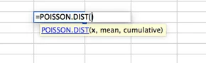
| Probability | =POISSON.DIST(A2,$B$1,FALSE) | Probability of exactly that count |
| Cumulative probability | =POISSON.DIST(A2,$B$1,TRUE) | Lookup boundary for random draws |
Here $B$1 holds lambda, the expected average event count for the period. If you expect 6 support tickets per hour, lambda is 6. The count column should continue until the cumulative probability is effectively 100%.
To simulate one trial, generate a random probability with RAND() and return the first count whose cumulative probability is at least that random number. In current Excel, XLOOKUP can do that cleanly:
=XLOOKUP(RAND(), cumulative_probability_range, count_range,,1)Older workbooks can use an approximate-match VLOOKUP table with explicit 0% and 100% boundaries. Repeat the trial for hundreds or thousands of rows, then summarize the simulated counts with AVERAGE, MIN, MAX, PERCENTILE.INC, and a histogram.
The key modeling choice is whether Poisson is actually appropriate. Use it for independent count events with a stable average rate. Do not use it for dollar amounts, percentages, durations, or bounded quantities where a normal, triangular, lognormal, or custom distribution better matches the business process.
Analyzing the Results
When analyzing Monte Carlo simulation results in Excel, I focus on understanding output data, performing sensitivity analysis, and visualizing outcomes. These steps help in assessing financial risks and predicting possible outcomes like expected profit and maximum profit.
Understanding Output Data
To analyze output data effectively, I first examine the range of outcomes, including the minimum and maximum profit. This helps me grasp the variability in potential results. I also look at the mean or average profit, which gives insight into expected outcomes under different scenarios.
I pay close attention to variance and skewness as they indicate how spread out and asymmetrical the data is. High variance means greater risk, while skewness lets me know if there are more favorable or unfavorable outcomes. By organizing this data, I can make better financial decisions and manage risks.
Performing Sensitivity Analysis
Sensitivity analysis is crucial for identifying how changes in input variables affect my results. This process involves adjusting key metrics like revenue to see how they impact profits. I look for variables that cause significant shifts in outcomes and prioritize these in my risk assessment.
For a structured approach, I might use Excel’s Data Tables to test different scenarios. This helps me pinpoint the drivers of financial risk and improve decision-making. Sensitivity analysis enhances uncertainty analysis by showing how sensitive my model is to changes, allowing for more robust risk management.
Visualizing Outcomes
Visualizing outcomes is essential for grasping the full picture. I use Excel charts to display a range of outcomes quickly. Histograms are great for showing the frequency of profit levels, making it easy to spot patterns.
I also use scatter plots to illustrate relationships between variables and outcomes. This allows me to see the potential spread of results and identify clusters or outliers. Visual tools aid in communicating results to stakeholders and enable clearer insights into potential scenarios. Tables or charts make complex data more approachable, leading to better decision-making.
Advanced Techniques and Tools
Exploring advanced Monte Carlo simulation techniques in Excel can enhance decision-making in areas like financial forecasting and risk analysis. I’ll cover optimizing simulations and integrating useful Excel add-ins.
Optimizing Simulations
In my experience, optimizing simulations can provide more accurate predictions. One way to achieve this is by fine-tuning inputs. For example, using tools like Stdev.P helps analyze variability, ensuring that simulated outcomes reflect real-life scenarios.
Applying mathematical techniques improves model reliability. Tackling problems related to production quantity or variable cost becomes easier with a precise simulation model. This method assists in data-driven decisions by clarifying potential risks and financial impacts.
Research supports that using these techniques can significantly improve risk analysis and decision support.
Using Excel Add-Ins
To enhance Monte Carlo simulations, Excel add-ins are invaluable. One useful tool is the Data Analysis ToolPak, which offers a straightforward interface to manage complex calculations.
Add-ins simplify creating simulations, analyze data trends, and refine forecasting models. They assist in running thousands of simulations efficiently, which is crucial for understanding variables impacting outcomes.
By integrating these tools, I can perform detailed risk analysis and improve the accuracy of my predictions. These resources expand Excel’s capabilities beyond basic functions, proving essential for those serious about financial modeling and decision-making.
What is the Monte Carlo Simulation?
Monte Carlo Simulation is a process of using probability curves to determine the likelihood of an outcome. You may scratch your head here and say… “Hey Rick, a distribution curve has an array of values. So how exactly do I determine the likelihood of an outcome?” And better yet, how do I do that in Microsoft Excel without any special add-ins
Thought you would never ask.
This is done by running the simulation thousands of times and analyzing the distribution of the output. This is particularly important when you are analyzing the output of several distribution curves that feed into one another.
Example:
- # of Units Sold may have a distribution curve
- multiplied by Market price, which may have another distribution curve
- minus variable wages which have another curve
- etc., etc.
Once all these distributions are intermingled, the output can be quite complex. Running thousands of iterations (or simulations) of these curve may give you some insights. This is particularly useful in analyzing potential risk to a decision.
Describe Monte Carlo
When describing Monte Carlo Simulation, I often refer to the 1980’s movie War Games, where a young Mathew Broderick (before Ferris Bueller) is a hacker that uses his dial up modem to hack into the Pentagon computers and start World War 3. Kind of. He then had the Pentagon computers do many simulations of the games Tic Tac Toe to teach the computer that no one will will a nuclear war – and save the world in the process.
Thanks Ferris. You’re a hero.
Here’s a glimpse of the movie to show you big time Monte Carlo in action. I am assuming that you will overlook the politics, the awkward man hugging and of course, Dabney Coleman.
The Monte Carlo Simulation Formula
Distribution Curves
There are various distribution curves you can use to set up your Monte Carlo simulation. And these curves may be interchanged based on the variable. Microsoft doesn’t have a formula called “Do Monte Carlo Simulation” in the menu bar 🙂
Uniform Distribution
In a uniform distribution, there is equal likelihood anywhere between the minimum and a maximum. A uniform distribution looks like a rectangle.
Normal (Gaussian) Distribution
This is also your standard bell shaped curve. This Monte Carlo Simulation Formula is characterized by being evenly distributed on each side (median and mean is the same – and no skewness). The tails of the curve go on to infinity. So this may not be the ideal curve for house prices, where a few top end houses increase the average (mean) well above the median, or in instances where there is a hard minimum or maximum. An example of this may be the minimum wage in your locale. Please note that the name of the function varies depending on your version.
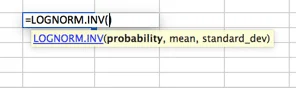
Lognormal Distribution
A distribution where the logarithm is normally distributed with the mean and standard deviation in Excel. So the setup is similar to the normal distribution, but please note that the mean and standard_dev variables are meant to represent the logarithm.
Poisson Distribution
This is likely the most underutilized distribution. By default, many people use a normal distribution curve when Poisson is a better fit for their models. Poisson is best described when there is a large distribution near the very beginning that quickly dissipates to a long tail on one side. An example of this would be a call center, where no calls are answered before second ZERO. Followed by the majority of calls answered in the first 2 intervals (say 30 and 60 seconds) with a quick drop off in volume and a long tail, with very few calls answered in 20 minutes (allegedly).
The purpose here is not to show you every distribution possible in Excel, as that is outside the scope of this article. Rather to ensure that you know that there are many options available for your Monte Carlo Simulation. Do not fall into the trap of assuming that a normal distribution curve is the right fit for all your data modeling. To find more curves, to go the Statistical Functions within your Excel workbook and investigate. If you have questions, pose them in the comments section below.
Building The Model
For this set up we will assume a normal distribution and 1,000 iterations.

Input Variables
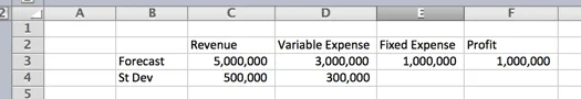
The setup assumes a normal distribution. A normal distribution requires three variables; probability, mean and standard deviation in Excel. We will tackle the mean and standard deviation in our first step. I assume a finance forecasting problem that consists of Revenue, Variable and Fixed Expenses. Where Revenue minus Variable Expenses minus Fixed Expenses equals Profit. The Fixed expenses are sunk cost in plant and equipment, so no distribution curve is assumed. Distribution curves are assumed for Revenue and Variable Expenses.

First Simulation
The example below indicates the settings for Revenue. The formula can be copy and pasted to cell D6 for variable expenses. For Revenue and expenses we you the function NORM.INV() where the parameters are:
- Probability = the function RAND() to elicit a random number based on the other criteria within the distribution.
- Mean = The mean used in the Step 1. For Revenue it is C3.
- Standard Deviation = The Standard Deviation used in Step 1. For Revenue it is C4
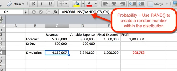
Since RAND() is used as the probability, a random probability is generated at refresh. We will use this to our advantage in the next step.

1,000 Simulations
There are several ways to do 1,000 or more variations. The simplest option is to take the formula from step #2 and make it absolute. Then copy and paste 1,000 times. That’s simple, but not very fancy. And if Ferris Bueller can save the world by showing a new Tic Tac Toe game to a computer, then we can spice up this analysis as well. Let’s venture into the world of tables.
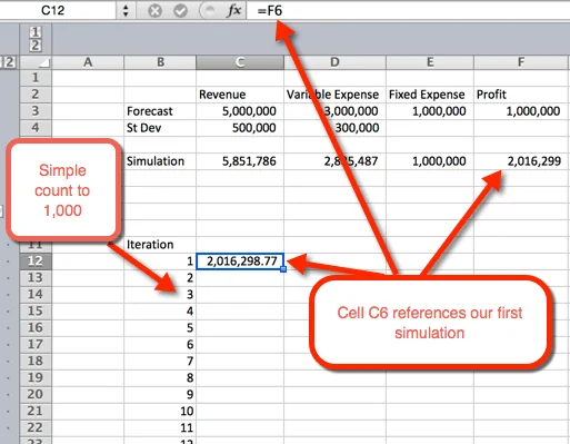
- First we want to create an outline for a table. We do this by listing the numbers 1 to 1,000 in rows. In the example image below, the number list starts in B12.
- in the next column, in cell C12, we will reference the first iteration.
- Next highlight the area where we want to house the 1,000 iterations
- Select Data > Data Tables
- For Column input cell: Select a blank cell. In the download file, cell D11 is selected
- Select OK
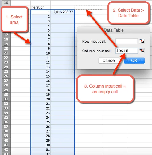
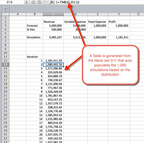
- Once OK is selected from the previous step, a table is inserted that autopopulates the 1,000 simulations

Summary Statistics
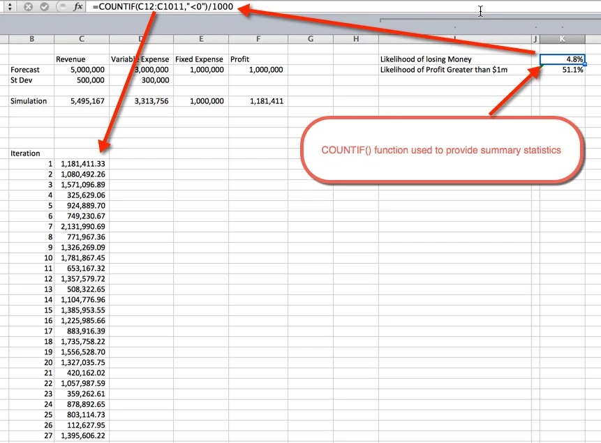
Once the simulations are run, it is time to gather summary statistics. This can be done a number of ways. In this example I used the COUNTIF() function to determine the percentage of simulations that are unprofitable, and the likelihood of a profit greater than $1 Million. As expected, the likelihood of greater than $1M hovers around 50%. This is because we used normal distribution curves that are evenly distributed around the mean, which was $1M. The likelihood of losing money is 4.8%. This was gathered by using the COUNTIF() function to count the simulations that were less than zero, and dividing by the 1,000 total iterations.
 Monte Carlo Simulation Formula
Get the Download
Conclusion
As I wrap up my exploration of the use of Monte Carlo Simulation in Excel, I find it invaluable for modeling uncertainty. With this tool, I can simulate various outcomes by running numerous scenarios, making it an essential strategy for risk analysis.
Excel proves to be a flexible platform for conducting these simulations. By using its built-in functions and abilities, I can efficiently manage data and forecast potential outcomes. Whether I’m simulating financial risks or predicting project timelines, Excel handles it well.
For larger simulations, using VBA code enhances efficiency by automating repetitive tasks. This is particularly helpful when dealing with thousands of scenarios.
Frequently Asked Questions
I often receive questions about how to effectively perform Monte Carlo simulations using Microsoft Excel. Below, I address some common inquiries, providing clear and practical insights.
How can you perform a Monte Carlo simulation in Microsoft Excel?
To perform a Monte Carlo simulation in Excel, I start by setting up a model with defined variables and formulas. Then, I generate random numbers for these variables and run the simulation multiple times. This way, I obtain a range of possible outcomes. For a step-by-step guide, refer to this resource.
What are the steps required to build a Monte Carlo simulation model in Excel?
Building a Monte Carlo simulation model involves several steps. Initially, I define the variables and metrics in Excel. I then use formulas to connect these metrics and simulate different scenarios. Running the simulation repeatedly allows me to analyze various possible outcomes, as highlighted in this detailed guide.
Are there any free tools available for conducting Monte Carlo simulations in Excel?
Excel itself acts as a useful tool for running Monte Carlo simulations without additional cost. However, there are third-party add-ins available that enhance the functionality. Tools like Data Tables and the RAND function in Excel provide capabilities to perform these simulations straightforwardly, as noted on DataCamp.
How do you incorporate probability distributions in a Monte Carlo simulation in Excel?
To incorporate probability distributions, I use Excel’s built-in functions. Functions like NORM.INV can create distributions based on means and standard deviations. This allows simulations to reflect realistic variations in data, enabling better decision-making.
What is the process for using Monte Carlo simulation for retirement planning in Excel?
For retirement planning, I construct a simulation to estimate different scenarios of savings and withdrawals over time. It involves projecting future rates of return, inflation, and other key factors to understand the impact on savings. By repeating these simulations, I get a clearer picture of potential financial outcomes during retirement.
Can Monte Carlo simulations be used for financial modeling in Excel, and if so, how?
Yes, Monte Carlo simulations are valuable for financial modeling. They help assess risk and forecast financial scenarios by running simulations with various inputs. These inputs can include changes in market conditions or interest rates. Excel’s robustness allows for detailed analysis, making it suitable for complex financial models.
Now What?
What have you used it for? Are there any specific examples that you can share with the group? If so, leave a note below in the comments section. Also, feel free to sign up for our newsletter, so that you can stay up to date as new Excel.TV shows are announced. Leave me a message below to stay in contact.

Comments (28)
Historical comments preserved from the WordPress archive. Commenting is no longer active.
Hi Rick – great post. One typo though – on second last line the copy should read “COUNTIF()” not “COUNTIT()”
Thanks Gerald. Correcting it now.
Maybe he wanted to count how tits Monte Carlo has seen
Hi Rick,
I have tried explaining what a basic Monte Carlo simulation is many times. I’m going to send them the link to your article from now on. Great summary!
Cheers,
Kevin
http://www.youtube.com/user/MySpreadsheetLab
Thanks Kevin. I cant tell you how many times I’ve told people “It’s like that movie War Games” and they just gave me that blank stare.
Hi Rick,
This is a very useful article and I’ve been able to employee the lessons learned in my own work. However, is there a way to record the randomly generated values used to calculate each case or iteration? For instance, what if in addition to finding the likelihood of losing money, I wanted to find the likelihood of losing money when Condition A is met, then Condition B, and so on? I think it would be easier to conditionally analyze a full table rather than generating a new Monte Carlo simulation for each condition.
Thanks,
Kevin
Great article and explanation of Monte Carlo simulation. That analogy to that scene in War Games is brilliant and makesbtotal sense.
I personally approve all comments where my analogies are called brilliant. 🙂
Hi Rick
Thank you for the lesson.
I have a question, which probably sounds STUPID.
When you have a distribution such as the Normal or LogNormal most of the data is close to the mean or mode etc. when you sample in say Excel what ensures that you are not giving equal weight to the tails where there is little data. Is it using the inverse function.
This has been bugging me for days. I’m trying to write a simulation for the effect of risk drivers in VBA (as per Dr David Hulett) on project estimates but I cannot find a proper explanation in the books I’ve consulted or else the level of math Stats is above the level that I used to understand 30 years ago. Thank You Braam Botha
Using some standard deviation within the inverse function tells Excel where you think most of the data lies
Rick,
I am a novice on monte carlos and only in the last week started learning as much as I can since I am interviewing for a job.
I would like one on one coaching on this. Would like your help.
Hi Rick, thanks for the great article. I have a question for you. I need to use the poisson distribution for my data since it’s definitely non-normal, however, Excel does not have the inverse function for Poisson as it does for the normal distribution (and some others). How would you recommend to work around this issue? Thanks
Hi Adam! (It’s Jordan!) Excel has a POISSION.DIST function in Excel 2013 and beyond. You could make the cumulative distribution and look up against it. Not my favorite solution but I’ll keep looking.
Hi Adam. I posted a new article on the Poisson distribution for Monte Carlo. Check it out. https://excel.tv/monte-carlo-simulation-excel-poisson-distribution/
Hi Rick,
I have a fairly complex model (hundreds of rows across multiple worksheets). I’d like to run monte carlo simulations on it by testing how the end results of the model vary when I vary one (or two or three) of the core input variables at a time.
This is more complex than the example in this article because I can’t calculate the end results just using a few cells – it takes multiple worksheets to produce the output.
I’m trying to extrapolate your example to my model, but I can’t figure it out yet. How can I simulate changing value G11 on Worksheet A then logging value G123 on Worksheet E a thousand times?
Thanks!
Hi Rick, please I need a little clarification concerning the countif function you used. Do you mean counting value obtained from iteration less than 1,000? because I can see any value less than zero
Thank you – very useful…
How do you do the simulation if you have a Poisson distribution? We need another article to cover this example. It would be useful.
Hi Dave – I created another article for Poisson.
https://excel.tv/monte-carlo-simulation-excel-poisson-distribution/
Hi Rick, thank you for providing such a great article on Monte Carlo (MC) simulation. I have read all the previous comments to make sure my simple question has not been answered elsewhere.
In the sample worksheet that I downloaded, the formula in cell K2 shows “=COUNTIF(C12:C1011,”1000000″)/1000”. As you can see, the row references in the formula in K2 capture 1000 rows beginning at C12 whereas the row references in the formula in K3 start at C11 so a different block of 1000 rows is captured. The difference between the two blocks of 1000 rows is very slight (1 row) and there is no appreciable differences in the values of K2 and K3 when “C12:C1011” is used in the formula in K3.
My question: is the starting row of C11 for the formula in K3 done on purpose or was a reason for this that I missed in the article (or maybe an unintentional copy and paste error)
Many thanks in advance for your clarification and again for providing such a clear example of how to use MS Excel for MC simulations.
Hi Rick, Thank you very much for this presentation. It has wet my appetite to research this topic further. You described the Monte Carlo simulation clearly which made it easy to understand and follow.
Cheers
Nadarajan
Excellent tutorial, perfect explanation! Thank you, very useful 🙂
Great article and the best explanation I found. Could you add more information on how the data table works to create the iterations? Thanks
If you do this and calculate the standard deviation of the numbers generated, it is not C4. It is generally materially higher than C4. Because the probabilities picked by RAND(0) are random you will pick numbers near the tail of the normal distribution more often than if the probability selection was itself normal. This seems to inflate the measured standard distribution. The mean is unaffected.
is there a program already set up in excel anywhere that can analyze data for tribal enrollment scenarios?