To freeze a row in Excel, keep the cursor on the worksheet, then use View > Freeze Panes and choose the option that matches what you want to keep visible. For the top row only, use Freeze Top Row or press Alt+W+F+R; for multiple rows, click the row below the last row you want frozen and choose Freeze Panes.
| Option | What It Does | Keyboard |
|---|---|---|
| Freeze Top Row | Freezes row 1 only | Alt+W+F+R |
| Freeze First Column | Freezes column A only | Alt+W+F+C |
| Freeze Panes | Freezes everything above/left of selected cell | Alt+W+F+F |
- How Freeze Panes Works
- How to Freeze the Top Row
- How to Freeze Multiple Rows
- How to Freeze Rows and Columns Together
- Excel for Web Differences
- Troubleshooting Common Issues
- FAQ
How Freeze Panes Works
Freeze Panes keeps part of a worksheet visible while the rest of the sheet scrolls. In practice, that usually means locking a header row at the top so column names stay on screen while you move through hundreds or thousands of records.
This is useful when managing finances, reviewing exported reports, or building visualization dashboards that pull from longer tables. The feature changes what you see while working in the sheet, but it does not change formulas, sort order, filter behavior, or print layout. If your worksheet is wide rather than tall, see how to freeze a column in Excel for the horizontal version of the same workflow.
Excel offers three related commands under the same menu:
- Freeze Top Row locks row 1.
- Freeze First Column locks column A.
- Freeze Panes locks everything above and to the left of the active cell.
That last command is the one to use when your headers span more than one row, or when you want row labels and column labels visible at the same time.
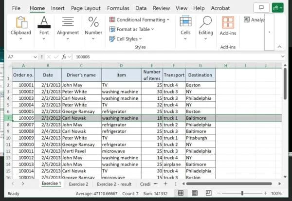
How to Freeze the Top Row
If your headers are in row 1, this is the fastest method.
- Open the worksheet you want to work in.
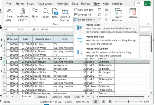
- Go to the View tab on the Excel ribbon.
- Select Freeze Panes.
- Choose Freeze Top Row.
Keyboard shortcut: Alt+W+F+R
After you turn it on, a thin line appears below row 1. Scroll down the sheet and row 1 stays in place while the remaining rows move underneath it.
This option is best when:
- Your worksheet has a single header row.
- The top row contains field names like Date, Customer, Amount, or Status.
- You want the quickest command without selecting any cells first.
 Excel Select a Row
One common mistake is selecting row 1 and then clicking Freeze Panes instead of Freeze Top Row. That does not freeze row 1 by itself. The dedicated Freeze Top Row command is the correct one when you only want the first row locked.
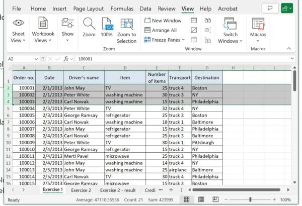
How to Freeze Multiple Rows
If your worksheet uses two or more header rows, use Freeze Panes rather than Freeze Top Row.
The rule is simple: click the row below the last row you want frozen.
For example:
- To freeze rows 1 and 2, click any cell in row 3.
- To freeze rows 1 through 3, click any cell in row 4.
- To freeze rows 1 through 10, click any cell in row 11.
Then follow these steps:
- Click any cell in the row below the rows you want to keep visible.
- Open View > Freeze Panes.
- Select Freeze Panes.
Keyboard shortcut: Alt+W+F+F
 Excel Freeze Pane
If the worksheet has title rows, merged report labels, or instructions at the top, check which row contains the labels you actually need during scrolling. Many users freeze too many rows at first, which leaves less room for the data itself. A practical approach is to freeze only the rows that identify the columns or define the section you are reviewing.
Example: Monthly Budget Sheet
Say row 1 contains a report title, row 2 contains the month, and row 3 contains the real column headers such as Category, Budget, Actual, and Difference. To keep all three visible, click row 4 and use Freeze Panes. That way the title and labels remain visible while you scroll through the transactions below.
 Excel Freeze Multiple Rows
How to Freeze Rows and Columns Together
Sometimes a sheet needs both horizontal and vertical reference points. A sales sheet might have product names in column A and months across row 1. In that case, freezing only the top row still leaves the row labels disappearing when you scroll to the right.
To freeze rows and columns together, click the cell directly below the rows you want frozen and directly to the right of the columns you want frozen.
Examples:
- Freeze row 1 and column A: click cell
B2. - Freeze rows 1 and 2 plus columns A and B: click cell
C3. - Freeze rows 1 through 3 plus column A: click cell
B4.
Then go to View > Freeze Panes > Freeze Panes or press Alt+W+F+F.
 Excel Freeze Rows and Columns
This works because Excel freezes everything above and left of the active cell. It does not freeze the selected cell itself. Keeping that rule in mind makes the feature much easier to use on the first try.
How to Unfreeze and Adjust Frozen Rows
If the wrong rows are frozen, or if you want to change the frozen area, remove the current setting first.
- Go to View.
- Select Freeze Panes.
- Choose Unfreeze Panes.
 Excel Adjusting Frozen Rows
After that, click the correct cell or row and apply the new freeze setting. Excel only keeps one freeze configuration at a time, so changing it always starts with Unfreeze Panes.
This matters when you receive a workbook from someone else. The sheet may already have a frozen area that does not match your needs, which makes the command look like it is not working. In many cases, nothing is broken; the current freeze just needs to be cleared first.
Keyboard Shortcuts for Freeze Panes
If you work in Excel all day, the ribbon path is fine, but shortcuts are faster once they become muscle memory.
- Freeze Top Row:
Alt+W+F+R - Freeze First Column:
Alt+W+F+C - Freeze Panes using the active cell:
Alt+W+F+F
These are Windows ribbon shortcuts. Press Alt, then the remaining letters in order. If you are working in Excel for Mac, the exact key sequence is different because Mac Excel does not use the same Alt ribbon navigation pattern.
Excel for Web Differences
Excel for Web also includes freeze options, but it is more limited than the desktop app. In the online version, go to View > Freeze Panes to open the dropdown.
The main difference is that Excel for Web supports freezing the top row or first column, but it does not support custom freeze pane selections the way the desktop app does. If you need to freeze multiple rows or freeze rows and columns together based on a selected cell, open the workbook in the desktop version of Excel.
That difference matters when a workbook moves between desktop and browser use. A custom freeze created in desktop Excel may not be something you can recreate from scratch in the web app, even though the workbook can still open online.
Protect-Sheet Gotcha
If Freeze Panes is unavailable or does nothing on a protected worksheet, check sheet protection before changing anything else.
Freeze Panes does not work when sheet protection is enabled. You must unprotect the sheet first through Review > Unprotect Sheet, then return to View > Freeze Panes and apply the setting you want.
If the workbook is shared by a team, you may need the password from the file owner before unprotecting the sheet.
Troubleshooting Common Issues
Most Freeze Panes problems come down to selection, worksheet state, or an existing freeze setting.
Freeze Panes Is Greyed Out
If the command is greyed out, Excel is often still in cell editing mode. Press Enter or Esc to exit editing, then try again.
Other quick checks:
- Click back into the worksheet if a chart, shape, or object is selected.
- Confirm the sheet is not protected.
- If the workbook is open in a limited environment, switch to the desktop app.
Freeze Panes Is Not Working
If the command runs but the result is not what you expected, check whether the sheet already has panes frozen. Use View > Freeze Panes > Unfreeze Panes, then apply the correct freeze again.
Also verify the active cell before using Freeze Panes. Excel freezes everything above and left of that cell, so clicking the wrong row or column changes the result immediately.
The Wrong Row Stayed Visible
This usually happens when Freeze Top Row was used instead of Freeze Panes, or when the active cell was too high in the sheet.
Use this quick rule:
- One header row in row 1: use Freeze Top Row.
- More than one row: click the row below them and use Freeze Panes.
Scrolling Feels Strange After Freezing
That is normal if several rows or columns are frozen. The visible area for scrolling becomes smaller because part of the window is permanently reserved for the frozen section. If it feels cramped, unfreeze and reduce the number of rows or columns you keep locked.
Version Notes for Excel Users
The general steps are similar across different versions of Excel, but the layout of the ribbon or menus may look a little different. The underlying behavior stays the same: Freeze Top Row locks row 1, Freeze First Column locks column A, and Freeze Panes locks everything above and left of the selected cell.
On mobile devices, the process can differ because the touch interface hides some ribbon commands behind menus. If you do not see the option right away, look for the View tab or open the workbook on desktop for full freeze pane controls.
FAQ
Can I freeze multiple rows and columns at the same time?
Yes. Click the cell below the last row you want frozen and to the right of the last column you want frozen, then use View > Freeze Panes > Freeze Panes.
Will freezing panes affect how my worksheet prints?
No. Freezing panes only affects what stays visible on screen while you scroll. It does not change the print layout.
Can I freeze panes in Excel Online?
Yes, but with limits. In Excel for Web, use View > Freeze Panes for the top row or first column. Custom pane freezing is not available there.
What happens if I freeze a row and then filter my data?
The frozen row remains visible while the filtered results below it change.
Is it possible to freeze rows at the bottom of the spreadsheet?
No. Excel only allows rows at the top and columns on the left to be frozen.
