
Strikethrough in Excel is the quickest way to cross out text without deleting it, and the best part is that it does not affect formulas, totals, or references. If you want to mark a task as done, show that a price has been replaced, or keep a historical value visible while making it clear that it is no longer current, strikethrough is the cleanest visual cue. The fastest way to apply it is Ctrl+5.
If you are pairing formatting styles, you may also want the companion guide on how to change text color and font in Excel. That post handles the rest of the font workflow, while this one focuses on the exact ways to cross out text and use the shortcut efficiently.
Stat block
On 2026-07-02, the content plan recorded strikethrough in excel at 12,100 monthly searches with KD 0. Microsoft also documents Ctrl+5 as the strikethrough shortcut in Excel, which is why this tiny formatting feature deserves a dedicated guide.
Source: content-strategy/blog-keyword-plan-2026-07.md · Microsoft Excel support
What strikethrough in Excel actually does
Strikethrough is a font effect that draws a line through text while leaving the cell value intact. In plain English, it says, “this is still here, but it is no longer the active version.” That makes it ideal when you need a visible audit trail, a revision history, or a quick way to compare old and new information without deleting anything.
I like strikethrough because it solves a very specific problem: deletion can be too final, but color alone can be too subtle. A crossed-out value tells the viewer, in one glance, that the item has changed. It works well for prices, tasks, inventory labels, spreadsheet notes, and any workflow where you want the original text to remain searchable and printable.
Here is the simplest way to think about it:
- Strikethrough is visual only. It changes how the text looks, not what the cell contains.
- It is reversible. You can turn it on and off with the same shortcut.
- It works on partial text. You can cross out just one word inside a cell.
- It scales well. You can use it in one cell or on an entire range.
If you need to communicate “old version” versus “new version” without adding extra columns, this is one of the most efficient formatting tools in Excel.
How to add strikethrough in Excel with Ctrl+5
The fastest answer is simple: select the cell or text, then press Ctrl+5. Excel applies strikethrough immediately, and pressing Ctrl+5 again removes it. That makes the shortcut the best option when you are reviewing a list quickly and want to mark items without stopping to open menus.
Here is the shortcut workflow I use most often:
- Select one or more cells.
- Press Ctrl+5.
- Check the result.
- Press Ctrl+5 again to toggle it off if needed.
On some laptops, the function row is mapped through the Fn key, so you may need Ctrl+Fn+5 instead. If the shortcut does not seem to work, test it on a standard desktop keyboard or open the Format Cells dialog to confirm that Excel itself is behaving normally.
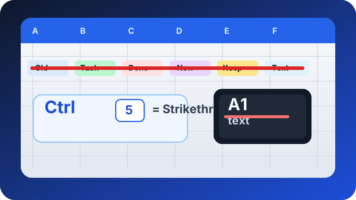
The shortcut also works on partial text inside a cell. That is useful when a line contains both active and inactive words, such as a note with a revised amount or a task that is partially complete. Double-click the cell, highlight the specific text, and then press Ctrl+5. Excel will only strike through the selected characters.
A few practical tips make this shortcut smoother:
- If you are editing a lot of cells, keep your left hand near Ctrl and your right hand near the number row.
- If the cell is in edit mode, select the text first, then use the shortcut.
- If a keyboard remapping tool is active, test the shortcut in a plain workbook before assuming Excel is the problem.
If you are building a repeatable workflow, the shortcut is hard to beat. It takes 1 gesture, preserves the cell contents, and keeps your worksheet readable while you review changes.
How to apply strikethrough through Format Cells
The Format Cells dialog is the best fallback when Ctrl+5 is not convenient or when you want to change multiple font settings at once. It gives you a clear checkbox for strikethrough and lets you combine the effect with bold, italic, font color, or underline in the same dialog.
Use this path:
- Select the cell or text.
- Press Ctrl+1 or right-click and choose Format Cells.
- Open the Font tab.
- Check Strikethrough.
- Click OK.
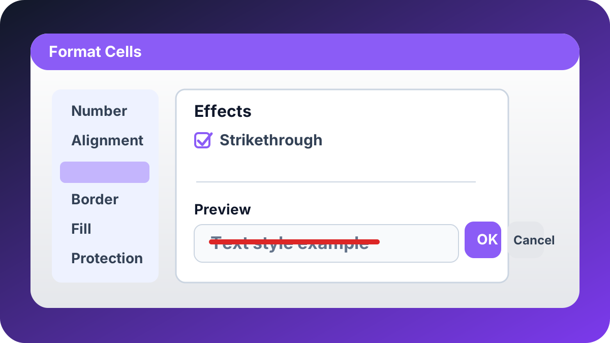
This method is especially helpful if you are already formatting the text for another reason. For example, you might want a crossed-out old price in gray italics while the new price stays bold and black. Doing all of that in one dialog is faster than applying each font effect separately.
It is also the cleaner option when you want to be precise about what changes. The dialog gives you a visible before-and-after preview, so you can confirm the result before you click OK. That matters when you are working in a sheet where the same font style appears in many places and you do not want accidental formatting changes.
A related scenario is conditional formatting. If you want Excel to strike through rows automatically when a status changes, you can build a rule that targets the font effect instead of manually toggling each cell. That approach is useful for task trackers, lists of completed items, or any spreadsheet where the state changes over time.
How to add strikethrough from the ribbon or Quick Access Toolbar
The ribbon is not the fastest path, but it is still useful when you prefer visible controls over keyboard shortcuts. You can reach strikethrough through the Font group, or you can add it to the Quick Access Toolbar so the command becomes a one-click action.
For the ribbon path, the practical route is:
- Select the text.
- Open Home.
- Launch the Format Cells dialog from the Font group.
- Check Strikethrough.
For the Quick Access Toolbar, I recommend this setup if you use strikethrough often:
- Right-click the ribbon.
- Choose Customize Quick Access Toolbar.
- Select All Commands.
- Find Strikethrough.
- Add it to the toolbar and click OK.
That gives you a permanent button for 1-click access. If you review revision lists every day, the toolbar route can save a surprising amount of time because you do not have to remember the shortcut or open the dialog each time.
The ribbon approach is also useful in training or shared-workbook environments. If you are showing someone else how the feature works, menu paths are often easier to demonstrate than a keyboard shortcut because the steps are visible on screen.
How to strike through only part of a cell
You can strikethrough only part of a cell by editing the cell, selecting the specific characters, and applying the format to just that selection. That is the best option when the cell contains a long note and only one phrase has changed, because the rest of the text stays readable and untouched.
Here is the pattern:
- Double-click the cell or press F2.
- Highlight the word or words you want to cross out.
- Press Ctrl+5.
This is much more precise than striking through the whole cell when only part of the text needs revision. I use it for comments like old price labels, corrected names, or notes where the original wording still matters for context.
The key thing to remember is that Excel treats the selected text like any other character formatting. That means you can combine partial strikethrough with bold, italic, or color changes if you need to show multiple states inside the same cell.
How to remove strikethrough in Excel
Removing strikethrough is usually easier than applying it. The direct method is to select the formatted cell or text and press Ctrl+5 again. Because the shortcut toggles the effect, it turns the line off immediately without changing any other font settings.
If you applied the effect through the Format Cells dialog, you can remove it the same way:
- Select the cell.
- Open Format Cells with Ctrl+1.
- Go to the Font tab.
- Uncheck Strikethrough.
- Click OK.
If you want to remove everything from the cell, use Home > Clear > Clear Formats. That is the blunt option, and I only use it when I want to strip all font changes, not just the crossed-out line.
One small troubleshooting tip: if the text still looks crossed out after you turn it off, check whether you selected the full range. Partial formatting can make it look like the effect is still active when only some characters were edited.
Best practices for using strikethrough well
Strikethrough works best when it has a clear meaning. If you use it randomly, it becomes visual noise. If you use it consistently, it becomes a reliable status signal that helps other people understand the workbook in 1 glance.
I follow a few rules:
- Use strikethrough for replaced, completed, or superseded text.
- Avoid using it for items that are merely “important” or “possible.”
- Pair it with a label or note if other people will view the workbook.
- Keep the formatting consistent across the sheet.
- Use it sparingly in dense tables so the sheet does not become hard to scan.
If you are managing prices, I recommend leaving the old price crossed out and putting the new price beside it. If you are tracking tasks, use one status convention across the workbook so strikethrough always means the same thing. If you are cleaning data, keep the row until the deletion is confirmed.
That last point matters more than it seems. A crossed-out item is still present in the file, so formulas, filters, and references can still see it. That is good for auditing, but it means you should not use strikethrough as a substitute for a real status field if the workbook needs logic downstream.
When strikethrough is better than deleting or recoloring
Strikethrough is the right choice when you want to preserve history. Deleting is better when the data truly should not exist anymore, and recoloring is better when you want to draw attention without implying that the item has been retired. Strikethrough sits in the middle: it says the text still matters, but not as the active version.
That makes it especially useful in shared workbooks. A teammate can see the old value, understand why it changed, and keep moving without digging through version history. It is also helpful in client-facing sheets, because crossed-out text feels more deliberate than a hard delete and more informative than a silent overwrite.
If you only need to change the appearance of text and not the data itself, strikethrough is usually the most honest formatting choice.
Quick comparison of the 3 main methods
| Method | Best for | Speed |
|---|---|---|
| Ctrl+5 | Fast editing and repetitive reviews | 1 step |
| Format Cells | Multiple font changes at once | 5 steps |
| Quick Access Toolbar | Frequent use without memorizing shortcuts | 1 click after setup |
The practical answer is simple: use Ctrl+5 most of the time, keep Format Cells as the fallback, and add the command to the Quick Access Toolbar if you use it every day.
Common mistakes to avoid
The most common mistake is assuming strikethrough changes the data value. It does not. The cell still contains the same text or number, so formulas keep working as usual.
A second mistake is striking through too much text. If only one word changed, edit the cell and apply the format just to that word. That keeps the worksheet easier to read.
A third mistake is using strikethrough as a permanent archive strategy in a sheet that still needs logical status tracking. If a record must be filterable, add a dedicated status column instead of relying on font effects alone.
Final takeaway
If you only remember 1 thing, remember this: Ctrl+5 is the fastest way to add or remove strikethrough in Excel, and it works whether you are crossing out a full cell or just a few selected words. Use Format Cells when you want more control, use the Quick Access Toolbar when you want a persistent button, and use strikethrough whenever the original text still matters.
If you are continuing your Excel formatting cleanup, the next logical step is how to change text color and font in Excel, because the two tools pair nicely when you need to show both “old vs. new” and “active vs. inactive” at the same time.
