Dynamic Project Cost Dashboard in Excel

This consolidated tutorial covers both the original VLOOKUP method and the automated reference-string method for building a dynamic project duration and cost dashboard in Excel.

Let’s say you are the manager of a portfolio of projects at your company.  While each project under your aegis is different, they have a few things in common; specifically – and for the sake of our example – they all go through (or, are currently in) three different phases, and each phase has a different cost per month, but the cost doesn’t differ between each project.  In our example, the phases are:

Phase Name Cost of each stage per month
1. Planning $250/month
2. Execution $500/month
3. Maturity $125/month

The idea is to capture both the cost in any given month and the overall cost over the life of the project.  For example, you have an IT Upgrades project in your portfolio.  You think that you will spend two months in Planning, nine months in Execution, and one month in Maturity after which the project will be closed.  Thus, the overall cost of your project is expected to be,

Planning @ two months: 2 months * $250 $/month  = $500
Execution @ nine months: 9 months * $500 $/month = $4500
Maturity @ one month: 1 month * $125 $/month = $125
Planning + Execution + Maturity =  $500 + $4500 + $125 = $5125

The problem is that each project is different.  One project might spend more time in the first phase than the other.  Moreover, for some projects you have a good idea of how long they will stay in each phase, and for some you are a bit less sure.  Boy, you say, wouldn’t it be nice to change how long a project stays in each phase to compare costs.  Wouldn’t it be nice to see it on a chart?  Let’s see what we can do.

Using a VLOOKUP might seem like an obvious choice for our solution.  Here’s how to do it.   
The Dynamic VLOOKUP Method

Step 1: Create the VLOOKUP table
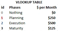
Since you know there are three projects, you could encode ids into a lookup table numbers as follows.

!

Step 2: Create a Reference Table
The Reference Table is a time-series table that holds the numerical references to your VLOOKUP table.  If IT Services has two months of Planning, then the Reference Table will show two 1’s in the first two months, respectively.

!

Step 3: Create a Values Table to map each reference to its monthly cost using VLOOKUP
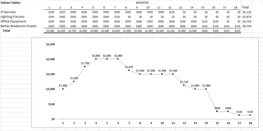
Now, you’ll make another table that is essentially a mirror image of your Reference Table. This table, however, maps each reference to the correct cost.  So, for Month 1 in the Values Table, VLOOKUP will use the corresponding reference (1) in the Reference Table to indicate the project is in the Planning phase and the associated cost is $250.

!

Step 4: Sum the Values Table, then graph

!

Summary
Our dynamic VLOOKUP() method works: the manager (that’s us) can replace the values in the Reference Table to update how long a project stays in each phase.  We would simply repeat numbers in the Reference Table in the amount of months a project is in a particular phase.  Our Values Table automatically updates based on each change.

So here’s the thing.  I don’t like this method at all.  For one, we need a VLOOKUP in for every month, for every program.  Our example only displayed a few projects in a small time frame, but the real world might have many projects over many years!  That’s a real problem because VLOOKUPs can become computationally expensive as our spreadsheet grows.

And there’s another problem, too.  The manager – that’s us, remember – must hand-jam the references in for every month. What if there are many years to account for?  We could Copy/Paste to make life easier, but this method is so very, very error-prone.  There should be a way for us to simply enter the months a project is in a given phase and have Excel automatically generate all the required reference information.

The VLOOKUP method works, but it still makes the user type a phase reference into every month. The next method removes that manual step.

Automated Method: Generate the Monthly References

When you know how many months each project stays in each phase, Excel can generate the reference pattern automatically. Instead of typing 1, 1, 2, 2, 2... month by month, the worksheet builds the string from the project inputs.

Step 1: Use REPT

REPT repeats a character a specified number of times. If A1 contains:

=REPT("A",6)

Excel returns AAAAAA. For this dashboard, the repeated character is the phase reference. If the project spends two months in Planning, the formula returns 11. If it spends nine months in Execution, it returns 222222222.

Step 2: Concatenate the Phase Strings

Use & to join the repeated Planning, Execution, and Maturity strings into one full project timeline. A project with 2 months of Planning, 9 months of Execution, and 1 month of Maturity would produce:

112222222223

Each character now represents one month in the project schedule.

Step 3: Use MID to Populate the Reference Table

MID reads one character at a time from the timeline string:

=MID(project_reference_string, month_number, 1)

Month 1 reads the first character, month 2 reads the second, and so on. When the month number is beyond the end of the string, MID returns blank, which is exactly what you want for months after the project has ended.

Step 4: Convert the Text References to Numbers

Because REPT and MID return text, convert each reference back to a number before using it in numeric formulas:

=VALUE(MID(project_reference_string, month_number, 1))

You can also use the double unary operator (--) if you prefer:

=--MID(project_reference_string, month_number, 1)

Step 5: Replace VLOOKUP with INDEX

Once each phase is encoded as 1, 2, or 3, INDEX is cleaner than VLOOKUP. Put the phase costs in a simple vertical list and use the generated phase number as the row argument:

=INDEX(phase_cost_range, phase_reference)

That maps Planning to the first cost, Execution to the second cost, and Maturity to the third cost without an approximate lookup table.

Step 6: Wrap Empty Months with IFERROR

Months outside the project schedule may return blanks or errors. Use IFERROR to force those months to zero cost:

=IFERROR(INDEX(phase_cost_range, phase_reference),0)

Step 7: Sum, Chart, and Add Conditional Formatting

After the Values Table returns monthly cost by project, sum each month and chart the result. You can also use the generated reference table for conditional formatting to create a simple Gantt-style view of the project phases.

The automated method is the better long-term model because the user only enters phase durations. Excel handles the monthly reference table, cost mapping, totals, and dashboard chart from those inputs.